
Vanadis 3D is an open-source, high-performance finite-element air pollution dispersion model for three-dimensional atmospheric advection–diffusion–reaction transport in prescribed velocity fields. Its spatial discretization uses Directional Residual (DR) stabilization, designed for advection-dominated, high-Peclet-number transport while retaining the physical diffusion operator in conventional Galerkin form. The solver also provides explicit global mass-balance diagnostics for quantitative verification of transient simulations.
Local element matrices [H] and [C] are constructed on the CPU and retained in Element-by-Element (EbE) form, without assembling a conventional global sparse matrix. The resulting algebraic system can be solved either on the CPU or with CUDA acceleration. The GPU implementation uses a parallel Element-by-Element iterative solver with lightweight diagonal preconditioning, allowing large three-dimensional transport problems to be handled with comparatively low memory requirements.
At the ground surface, Vanadis supports either a Dirichlet boundary condition or a Robin-type flux/deposition condition governed by the transfer coefficient α. Time integration uses an implicit A-stable scheme with θ = 2/3. At each time step, element matrices and right-hand-side contributions are evaluated locally and the resulting system is solved iteratively. The same formulation supports transient emissions Q(t), spatially and temporally varying transport fields, and concentration-dependent reaction or removal terms P(S).
The source code of the Vanadis solver is distributed under a dual‑license model (GPL‑3.0 + Commercial License). The GitHub repository provides the public source-code history, versioned releases, technical documentation, and ongoing development of the Vanadis model. Users who wish to extend or experiment with the solver may do so by copying the ZIP archive into their own environment.
This work is accepted as an oral presentation at the 25th Annual CMAS Conference, Chapel Hill, NC, October 2026 (/releases/tag/v2026.2.1). https://www.cmascenter.org/conference/2026/agenda.cfm
GIT repo: GitHub
The current formulation (/releases/tag/v2026.3.0) also supports a nonlinear concentration-dependent reaction/decay coefficient P(S), evaluated locally at the finite-element level. The resulting nonlinear system is solved using Picard iteration at each time step while preserving the existing Element-by-Element solution strategy.
The source-term formulation has also been generalized to support time-dependent emissions Q(t). Source strength is evaluated separately at the previous and current time levels, allowing temporally varying emission profiles to be represented. The current test case uses a constant source active from the initial time t=0.
The implicit time-integration scheme has been extended consistently to account for both the nonlinear reaction term and the time-dependent source contribution.
Technical documentation v2026.3.0
Patent application
Patent application P.455475 received an unfavorable preliminary assessment from the Polish Patent Office in July 2026 due to insufficient technical disclosure in the submitted documentation. Novelty and inventive step were not assessed. The Vanadis source code was made publicly available on GitHub only after the patent application had been filed.

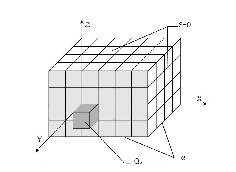
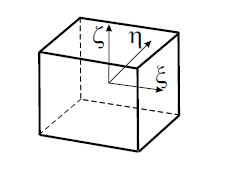
Geometry: The model uses linear 8‑node hexahedral elements with standard shape functions Ni, which provide trilinear interpolation of geometry and field variables within each element.
Weighting functions: The weighting functions in the weak formulation are the Directional Residual (DR) functions, which provide a local, streamline-oriented stabilization of the advective transport operator. Unlike standard Galerkin weighting, the DR formulation modifies the test functions in the direction of advection while retaining the Element-by-Element structure of the discretization.
Shape functions (interpolation): The scalar field S(x,y,z) is interpolated using the standard trilinear basis
Linear equations:
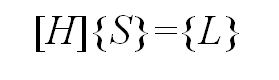
Steady state solution:
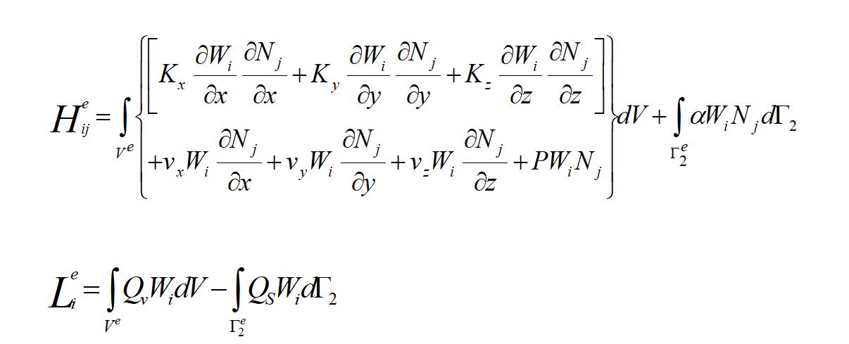
Dynamic solution:
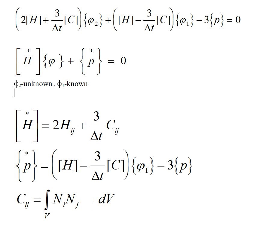
Time integration is performed using an implicit time-discrete formulation originating from numerical-methods lectures at AGH University of Science and Technology (Prof. Maciej Pietrzyk, ca. 1995). In the considered atmospheric dispersion simulations, the scheme demonstrated robust numerical stability and reliable iterative convergence for time steps of 100 s. Its ability to operate with relatively large time steps contributes substantially to the computational efficiency of large-scale transient advection-diffusion simulations.
.
This consistent transient-advection coupling is a fundamental part of the DR formulation rather than an implementation detail.
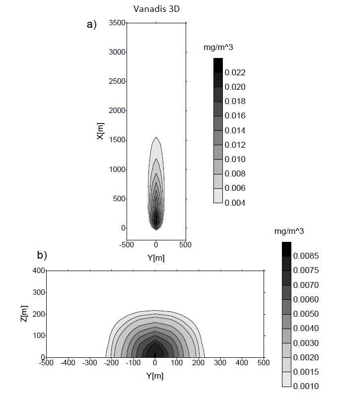
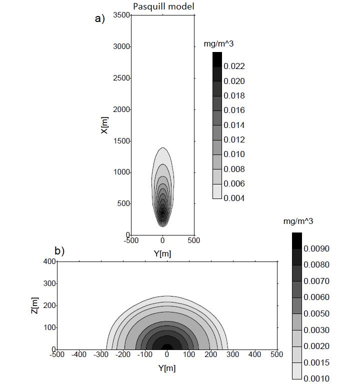
Vanadis runs on Linux or Windows systems and requires a Fortran compiler for building the CPU version of the solver. GPU acceleration is optional and uses the NVIDIA CUDA Toolkit.
For a representative test case consisting of approximately 2.8 million nodes and a 100-second time step, the following performance was observed:
CPU (Intel Core i5-4590 @ 3.30 GHz, 4 GB RAM): approximately 20 seconds to solve the linear system for a single time step.
GPU (NVIDIA GTX 1060, 3 GB): approximately 10 seconds to solve the linear system for a single time step.
These results illustrate the computational efficiency of the GPU-accelerated Element-by-Element solver compared with the single-core CPU implementation.
For the same large-grid case (approximately 2.8 million nodes), the Vanadis solver completes a 2,000-second transient simulation in approximately 20 minutes.


The results are visualized on two orthogonal surfaces: the ground surface and a vertical cross‑section. At time t=0 the first chimney is activated. After 1000 seconds the second chimney is switched on and the wind direction is changed. The influence of the tall building on the flow field and pollutant dispersion is clearly visible.

Precompiled Windows demo — no source-code compilation required
3D transient advection–diffusion–reaction model
Time step: 100 s
Pollution source: one emitter located at (x = 0 m, y = 0 m, h = 60 m)
Domain size: 8000 m × 8000 m × 420 m (height)
Example output: ground‑level concentration after 2000 s (shown on the left)
Data availability: full output for every time step on all visualization surfaces
Adjustable parameters:
Qv [kg/s] — emission rate
Kx, Ky, Kz [m²/s] — turbulent diffusion coefficients
P [1/s] — decay constant
vh [m/s] — vertical wind component
vx, vy [m/s] — horizontal wind components
α [m/s] — deposition / settling parameter
author: Marek Chodorski
e-mail: marek_ac@wp.pl